Outcomes of Linear Programming Review

Unboundedness Review

We say a linear program with a minimization objective is unbounded if there are feasible points whose objective value can be made arbitrarily small.

If it has a maximization objective, then we would want the objective to be made arbitrarily large.

That is to say that for any number $t$, there is a feasible point with objective value less than $t$.

Unboundedness Review

Boundedness is a property of the whole linear program, not just the constraints.

Outcomes of Linear Programs

Outcomes of Linear Programs

For LP $\min c^{\intercal} x$ s.t. $Ax \le b$, each outcome has a certificate.

Infeasible

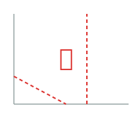
Certificate:

\[\begin{aligned}y &\ge 0\\A^{\intercal} y &= 0\\b^{\intercal} y &< 0\end{aligned}\]

Has an optimal point

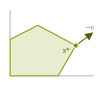
Certificate:

A feasible $x^*$ and

\[\begin{aligned}y &\ge 0\\A^{\intercal} y &= -c^{\intercal}\\b^{\intercal} y &= -c^{\intercal} x^*\end{aligned}\]

Unbounded

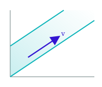
Certificate:

A feasible $x$, and

\[\begin{aligned}Av &\le 0\\c^{\intercal} v &< 0\end{aligned}\]

An Unbounded LP

Imagine adding one to every $x_i$. This keeps all of the constraints valid, and decreases the objective.

Therefore, this LP is unbounded. I can make the objective as small as I want while staying feasible.

An Unbounded LP

In matrix form, with $c = (-1,-1,-1)$, \[ A = \begin{pmatrix} 1 & -1 & 0 \\ 0 & 1 & -1 \\ -1 & 0 & 0\end{pmatrix}, \qquad b = \begin{pmatrix} 1 \\ 1 \\ 0\end{pmatrix}. \]

An Infeasible LP

The last three constraints say $x_1, x_2, x_3 \ge 0$, so $x_1 + x_2 + x_3 \ge 0$.

But the first constraint asks for $x_1 + x_2 + x_3 \le -1$. No point can satisfy both, so the LP is infeasible.

An Infeasible LP

Another perspective: If we add together all of the constraints, we get \[ (x_1+x_2+x_3) - x_1 - x_2 - x_3 \le -1 + 0 + 0 + 0. \] or $0 \le -1$, which is an invalid result.

An Infeasible LP

In matrix form, \[ A = \begin{pmatrix} 1 & 1 & 1 \\ -1 & 0 & 0 \\ 0 & -1 & 0 \\ 0 & 0 & -1\end{pmatrix}, \qquad b = \begin{pmatrix} -1 \\ 0 \\ 0 \\ 0\end{pmatrix}. \]

An LP with an Optimal Point

Minimizing $-x_1-x_2-x_3$ is the same as maximizing $x_1 + x_2 + x_3$.

Each constraint caps a variable at $1$, so $x_1 + x_2 + x_3 \le 3$, with equality at $x^* = (1,1,1)$. So $x^*$ is optimal, with value $-3$.

An LP with an Optimal Point

In matrix form, with $c = (-1,-1,-1)$, \[ A = \begin{pmatrix} 1 & 0 & 0 \\ 0 & 1 & 0 \\ 0 & 0 & 1\end{pmatrix}, \qquad b = \begin{pmatrix} 1 \\ 1 \\ 1\end{pmatrix}. \]

Standard Equality Form

Standard Equality Form

In the textbook, LPs are written in standard equality form.

Different forms of LPs are like different ways of writing fractions; they look different but are essentially the same.

Standard Equality Form

Geometric Perspective on SEF

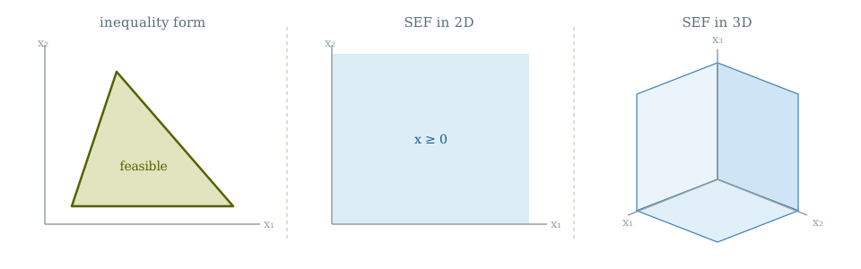
SEF starts from the nonnegative orthant $x \ge 0$.

Geometric Perspective on SEF

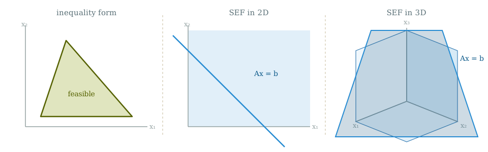
Overlay the affine subspace given by $Ax = b$.

Geometric Perspective on SEF

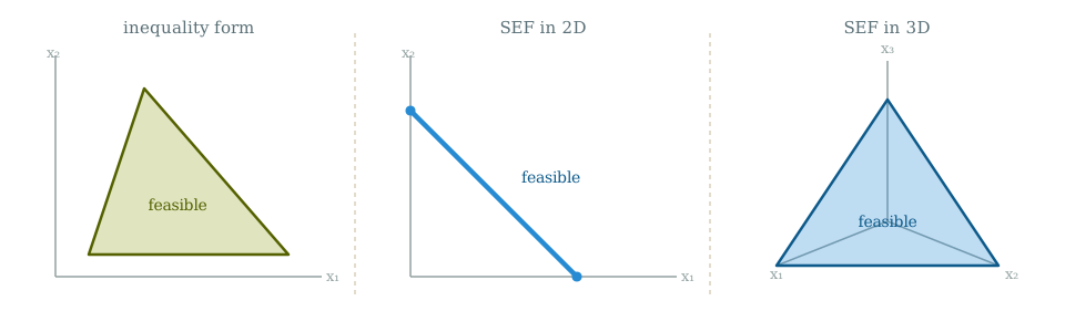
The feasible region is the part of $Ax = b$ lying in the orthant $x \ge 0$.

Standard Equality Form

Contrast with the form we have been using so far

Standard Equality Form

Example: Consider the following LP, not in SEF.

How to put this in SEF?

Standard Equality Form

Example: Consider the following LP, not in SEF.

Step 1: Use negation if necessary to replace make all of the inequalities less than or equal to, and also make the objective maximization.

Standard Equality Form

Example: Consider the following LP, not in SEF.

Step 1: Use negation if necessary to replace make all of the inequalities less than or equal to, and also make the objective maximization.

Standard Equality Form

Example: Consider the following LP, not in SEF.

Step 1: Use negation if necessary to replace make all of the inequalities less than or equal to, and also make the objective maximization.

Standard Equality Form

Example: Consider the following LP, not in SEF.

Step 2: Introduce nonnegative slack variables (one for each inequality) to take out the slack.

Standard Equality Form

Example: Consider the following LP, not in SEF.

Step 2: Introduce nonnegative slack variables (one for each inequality) to take out the slack.

Standard Equality Form

Example: Consider the following LP, not in SEF.

Step 2: Introduce nonnegative slack variables (one for each inequality) to take out the slack.

Standard Equality Form

Example: Consider the following LP, not in SEF.

Step 3: Replace each $x_i$ which does not need to be nonnegative with the difference of two new variables $x_{i}^+$ and $x_i^-$.

Standard Equality Form

Example: Consider the following LP, not in SEF.

Step 3: Replace each $x_i$ which does not need to be nonnegative with the difference of two new variables $x_{i}^+$ and $x_i^-$.

Standard Equality Form

Example: This LP is now in SEF (and equivalent to the original)

Standard Equality Form

More general schematic:

First apply step 1 of negating inequalities/objective to bring the LP in the following form:

for an $m\times n$ matrix $A$.

Standard Equality Form

More general schematic:

Step 2 is to introduce $s \in \R^m$ nonnegative slack variables to absorb the slack.

Standard Equality Form

More general schematic:

Step 3 is to replace all of the $x_i$'s with differences of nonnegative variables:

At this point, the LP is in SEF, though we can do one more step to make it a little clearer:

Standard Equality Form

is equivalent to

where we think of $z = \begin{pmatrix}x^+\\x^-\\s\end{pmatrix}$, $c' = \begin{pmatrix}c \\ -c \\ 0\end{pmatrix}$ and $A' = \begin{pmatrix}A & - A & I\end{pmatrix}$.

Standard Equality Form

Another example. Here $x_2 \ge 0$ but $x_1$ is free.

Standard Equality Form

Step 1: make the objective a max and every inequality a $\le$ (negating where needed). The equality stays as is.

Standard Equality Form

Step 2: add a slack variable to each inequality. The equality $x_1 + 2x_2 = 5$ needs no slack.

Standard Equality Form

Step 3: replace only the free variable $x_1$ with $x_1^+ - x_1^-$. Since $x_2 \ge 0$ already, it is left alone.

Standard Equality Form

This LP is now in SEF.

Certificates for SEF LPs

Outcomes of Linear Programs

For LP $\max c^{\intercal} x$ s.t. $Ax = b, x\ge 0$, each outcome has a certificate.

Infeasible

Certificate: a free $y$ with

\[\begin{aligned}A^{\intercal} y &\ge 0\\b^{\intercal} y &< 0\end{aligned}\]

Has an optimal point

Certificate:

A feasible $x^*$ and a free $y$ with

\[\begin{aligned}A^{\intercal} y &\ge c\\b^{\intercal} y &= c^{\intercal} x^*\end{aligned}\]

Unbounded

Certificate:

A feasible $x$, and a $v$ with

\[\begin{aligned}Av &= 0\\v &\ge 0\\c^{\intercal} v &> 0\end{aligned}\]

Outcomes of Linear Programs

Study Strategy: Space/Time tradeoff

One approach to learning about these certificates is just to remember all of the different definitions.

Another approach is to not memorize any of these definitions, but be able to derive each notion from scratch.

My suggestion: Remember the different certificates for the LPs in SEF, and then remember the different transformations that get you from any LP to that form.

Bases and Canonical Forms

Bases and Canonical Forms

Given a LP in SEF, some symmetries become visible that might not have been obvious before.

Bases and Canonical Forms

Example: \[ \begin{pmatrix} 1 & 2 & 3 \\ 4 & 5 & 6\end{pmatrix} \begin{pmatrix}x_1\\x_2\\x_3\end{pmatrix} = \begin{pmatrix} 1 \\ 0\end{pmatrix} \]

We can apply row operations to change the form of these linear equations.

Bases and Canonical Forms

Example: \[ \begin{pmatrix} 1 & 2 & 3 \\ 4 & 5 & 6\end{pmatrix} \begin{pmatrix}x_1\\x_2\\x_3\end{pmatrix} = \begin{pmatrix} 1 \\ 0\end{pmatrix} \] \[ \downarrow_{\rho_2 - 4 \rho_1}\] \[ \begin{pmatrix} 1 & 2 & 3 \\ 0 & -3 & -6\end{pmatrix} \begin{pmatrix}x_1\\x_2\\x_3\end{pmatrix} = \begin{pmatrix} 1 \\ -4 \end{pmatrix} \]

Note that even though we change the form of the linear system, the solutions stay the same. In particular, any nonnegative solution to the first system is a nonnegative solution to the second (and vice versa).

Bases and Canonical Forms

Example:

Further row operations reduce the problem to Row Reduced Echelon Form (RREF)

\[ \begin{pmatrix} 1 & 2 & 3 \\ 0 & -3 & -6\end{pmatrix} \begin{pmatrix}x_1\\x_2\\x_3\end{pmatrix} = \begin{pmatrix} 1 \\ -4 \end{pmatrix} \] \[ \downarrow_{\rho_2 / -3}\] \[ \begin{pmatrix} 1 & 2 & 3 \\ 0 & 1 & 2\end{pmatrix} \begin{pmatrix}x_1\\x_2\\x_3\end{pmatrix} = \begin{pmatrix} 1 \\ 4/3 \end{pmatrix} \]

Bases and Canonical Forms

Example:

Further row operations reduce the problem to Row Reduced Echelon Form (RREF)

\[ \begin{pmatrix} 1 & 2 & 3 \\ 0 & 1 & 2\end{pmatrix} \begin{pmatrix}x_1\\x_2\\x_3\end{pmatrix} = \begin{pmatrix} 1 \\ 4/3 \end{pmatrix} \] \[ \downarrow_{\rho_1 - 2 \rho 2}\] \[ \begin{pmatrix} 1 & 0 & -1 \\ 0 & 1 & 2\end{pmatrix} \begin{pmatrix}x_1\\x_2\\x_3\end{pmatrix} = \begin{pmatrix} -5/3 \\ 4/3 \end{pmatrix} \]

Bases and Canonical Forms

\[ \begin{pmatrix} 1 & 0 & -1 \\ 0 & 1 & 2\end{pmatrix} \begin{pmatrix}x_1\\x_2\\x_3\end{pmatrix} = \begin{pmatrix} -5/3 \\ 4/3 \end{pmatrix} \]

This system of equations tells us that $x_1 = -\frac{5}{3} + x_3$ and $x_2 = \frac{4}{3} - 2x_3.$

Bases and Canonical Forms

Example: An alternative perspective: If $Ax = b$, then for any invertible matrix $R$, we have that $RAx = Rb$ is an equivalent linear system.

\[ \begin{pmatrix} 1 & 2 & 3 \\ 4 & 5 & 6\end{pmatrix} \begin{pmatrix}x_1\\x_2\\x_3\end{pmatrix} = \begin{pmatrix} 1 \\ 0\end{pmatrix} \]

Bases and Canonical Forms

Example: An alternative perspective: If $Ax = b$, then for any invertible matrix $R$, we have that $RAx = Rb$ is an equivalent linear system.

\[ \begin{pmatrix}1 & 2 \\ 4 & 5 \end{pmatrix}^{-1}\begin{pmatrix} 1 & 2 & 3 \\ 4 & 5 & 6\end{pmatrix} \begin{pmatrix}x_1\\x_2\\x_3\end{pmatrix} = \begin{pmatrix}1 & 2 \\ 4 & 5 \end{pmatrix}^{-1}\begin{pmatrix} 1 \\ 0\end{pmatrix} \]

Bases and Canonical Forms

Example: An alternative perspective: If $Ax = b$, then for any invertible matrix $R$, we have that $RAx = Rb$ is an equivalent linear system.

\[ -\frac{1}{3}\begin{pmatrix}5 & -2 \\ -4 & 1 \end{pmatrix}\begin{pmatrix} 1 & 2 & 3 \\ 4 & 5 & 6\end{pmatrix} \begin{pmatrix}x_1\\x_2\\x_3\end{pmatrix} = -\frac{1}{3}\begin{pmatrix}5 & -2 \\ -4 & 1 \end{pmatrix}\begin{pmatrix} 1 \\ 0\end{pmatrix} \]

Bases and Canonical Forms

Example: An alternative perspective: If $Ax = b$, then for any invertible matrix $R$, we have that $RAx = Rb$ is an equivalent linear system.

\[ \begin{pmatrix} 1 & 0 & -1 \\ 0 & 1 & 2\end{pmatrix} \begin{pmatrix}x_1\\x_2\\x_3\end{pmatrix} = \begin{pmatrix} -5/3 \\ 4/3 \end{pmatrix} \]

Bases and Canonical Forms

Row reduction seems to make the first few coordinates seem more important than the other ones.

We can row reduce with respect to a different set of columns.

Bases and Canonical Forms

Example: Let us instead reduce with respect to columns $1$ and $3$. \[ \begin{pmatrix} \color{red}1 & 2 & \color{red}3 \\ \color{red}4 & 5 & \color{red}6\end{pmatrix} \begin{pmatrix}x_1\\x_2\\x_3\end{pmatrix} = \begin{pmatrix} 1 \\ 0\end{pmatrix} \]

We apply row operations to reduce the highlighted columns.

Bases and Canonical Forms

Example: \[ \begin{pmatrix} \color{red}1 & 2 & \color{red}3 \\ \color{red}4 & 5 & \color{red}6\end{pmatrix} \begin{pmatrix}x_1\\x_2\\x_3\end{pmatrix} = \begin{pmatrix} 1 \\ 0\end{pmatrix} \] \[ \downarrow_{\rho_2 - 4 \rho_1}\] \[ \begin{pmatrix} \color{red}1 & 2 & \color{red}3 \\ \color{red}0 & -3 & \color{red}{-6}\end{pmatrix} \begin{pmatrix}x_1\\x_2\\x_3\end{pmatrix} = \begin{pmatrix} 1 \\ -4 \end{pmatrix} \]

As before, the solution set is unchanged by row operations.

Bases and Canonical Forms

Example:

We reduce with respect to columns $1$ and $3$.

\[ \begin{pmatrix} \color{red}1 & 2 & \color{red}3 \\ \color{red}0 & -3 & \color{red}{-6}\end{pmatrix} \begin{pmatrix}x_1\\x_2\\x_3\end{pmatrix} = \begin{pmatrix} 1 \\ -4 \end{pmatrix} \] \[ \downarrow_{\rho_2 / -6}\] \[ \begin{pmatrix} \color{red}1 & 2 & \color{red}3 \\ \color{red}0 & 1/2 & \color{red}1\end{pmatrix} \begin{pmatrix}x_1\\x_2\\x_3\end{pmatrix} = \begin{pmatrix} 1 \\ 2/3 \end{pmatrix} \]

Bases and Canonical Forms

Example:

We reduce with respect to columns $1$ and $3$.

\[ \begin{pmatrix} \color{red}1 & 2 & \color{red}3 \\ \color{red}0 & 1/2 & \color{red}1\end{pmatrix} \begin{pmatrix}x_1\\x_2\\x_3\end{pmatrix} = \begin{pmatrix} 1 \\ 2/3 \end{pmatrix} \] \[ \downarrow_{\rho_1 - 3 \rho_2}\] \[ \begin{pmatrix} \color{red}1 & 1/2 & \color{red}0 \\ \color{red}0 & 1/2 & \color{red}1\end{pmatrix} \begin{pmatrix}x_1\\x_2\\x_3\end{pmatrix} = \begin{pmatrix} -1 \\ 2/3 \end{pmatrix} \]

Bases and Canonical Forms

\[ \begin{pmatrix} \color{red}1 & 1/2 & \color{red}0 \\ \color{red}0 & 1/2 & \color{red}1\end{pmatrix} \begin{pmatrix}x_1\\x_2\\x_3\end{pmatrix} = \begin{pmatrix} -1 \\ 2/3 \end{pmatrix} \]

Now $x_2$ is the free coordinate: $x_1 = -1 - \frac{1}{2}x_2$ and $x_3 = \frac{2}{3} - \frac{1}{2}x_2.$

Bases and Canonical Forms

Can we row reduce with respect to any set of columns?

A basis (plural bases) of a linear system is a set of columns of the matrix which are linearly independent, and where no larger set of columns is linearly independent.

For example, consider $A = \begin{pmatrix} 1 & 1 & 2 & 0 \\ 2 & 0 & 4 & 1\end{pmatrix}$. A basis is a set of two columns that are linearly independent.

Most pairs of columns form a basis, for instance \[ \{1,2\},\qquad \{2,3\},\qquad \{3,4\}. \]

But $\{1,3\}$ is not a basis: column $3$ is twice column $1$, so those columns are linearly dependent.

Bases and Canonical Forms

Can we row reduce with respect to any set of columns?

A basis (plural bases) of a linear system is a set of columns of the matrix which are linearly independent with as many columns as possible.

A variable is basic if it is part of the basis, and nonbasic if it is not.

The row reduced echelon form (RREF) of a linear system with respect to a basis is the result of row reducing system with respect to that basis.

Bases and Canonical Forms

Consider the system $Ax = b$ with \[ A = \begin{pmatrix} 1 & 2 & 3 & 1 \\ 1 & 2 & 3 & 0\end{pmatrix}, \qquad b = \begin{pmatrix} 4 \\ 1 \end{pmatrix}. \]

Columns $1, 2, 3$ are all parallel, so the only bases are $\{1,4\}$, $\{2,4\}$, and $\{3,4\}$: three canonical forms.

Bases and Canonical Forms

The three RREFs of $Ax = b$:

Bases and Canonical Forms

A basis for a LP corresponds to a set of variables (which also correspond to a column of $A$). A variable is said to be basic if it is part of the basis, and nonbasic otherwise.

Bases and Canonical Forms

For a linear program in SEF

We can replace the linear system with a RREF without changing the LP.

We can also change the objective!

Bases and Canonical Forms

Rewriting the objective

Consider

Bases and Canonical Forms

Rewriting the objective

Consider

Bases and Canonical Forms

If a linear system is in RREF, then we have essentially solved for the basic variables in terms of the nonbasic variables.

So we can backsubstitute for the basic variables in terms of the nonbasic variables in the objective.

Bases and Canonical Forms

If a linear system is in RREF, then we have essentially solved for the basic variables in terms of the nonbasic variables.

So we can backsubstitute for the basic variables in terms of the nonbasic variables.

Bases and Canonical Forms

If a linear system is in RREF, then we have essentially solved for the basic variables in terms of the nonbasic variables.

So we can backsubstitute for the basic variables in terms of the nonbasic variables.

Bases and Canonical Forms

A linear program in SEF is in canonical form with respect to a basis if the linear system $Ax = b$ is in RREF with respect to that basis, and the objective does not depend on the basic variables.

Bases and Canonical Forms

A linear program in SEF is in canonical form with respect to a basis if the linear system $Ax = b$ is in canonical form with respect to that basis.

Bases and Canonical Forms

A basic solution to a linear system is a solution where every nonbasic variable is equal to 0.

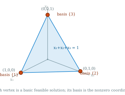
A basic solution which is feasible for an LP corresponds geometrically to a vertex of the feasible region!

Bases and Canonical Forms

Consider the SEF LP with the single constraint $x_1 + x_2 + x_3 = 1$ and $x \ge 0$. Its feasible region is a triangle, and each vertex is a basic feasible solution.

Bases and Canonical Forms

Equivalently, any linear function that is bounded on a polytope will have a minimum which is a vertex of the polytope.